**Note, for the TL;DR types, you can skip to the very bottom
for some graphs that demonstrate the answer to this question. This will be a
very long post. But the short answer is pretty worthless. And even as long as
this post is, it really should be longer. This still is just scratching the
surface.**
A few years back, I wrote a couple posts about some of the
basics of probability theory as it pertains to dice. In that, I reference the “Law
of Large Numbers” (LLN). Basically, as the number of experiments increases, the
average of the outcomes will approach the expected values.
So, how many dice does it take to make a large enough
sample? The simple answer – a lot.
I have heard some people state that they don’t ‘believe’ in
statistics as an application in games. I doubt such statements are meant
literally, but the explanation that follows often refers to the observation
that when a quantity of dice is rolled, the outcome usually does not ‘match’
the theoretical probability. Actually, this is completely as expected if you
understand statistics and combinatorics.
For example, since I know that each number on a D6 is
equally likely, if I roll 6 dice, I might expect to see one each of
1,2,3,4,5,6. In fact, this outcome is far less likely than having 5 numbers
with one repeated. I think I should save the mathematical explanation of that for
another time, as this is already going to be a very long post. But I do plan to
get to it soon-ish.
For this post, I will present the results of a few
simulations to try and illustrate this point. However, the fact is that most
game events will not require an amount of dice that comes anywhere near “large”.
So does this mean that theoretical probability is useless for game strategy?
Not exactly. But that explanation will need a lot of expansion, far more than I
can cover in one post. So, the examples that will be presented now are just an
introduction. We’ll see how this topic progresses, as I plan to return to it
often.
Some basic concepts used here:
“Error” refers to the degree by which an observed outcome (empirical
data) differs from the expected/theoretical value. In examples below, I may use
the term ‘difference’ instead of error as it seems more natural in this
context.
“Distribution” describes the ‘shape’ of data or expected
values. This is not necessarily confined to graphical representations, but it
makes concepts a bit more concrete if there is some picture to refer to. I am
actually using a very loose definition of distribution here, as it can include
many different specifications, but the full explanation on this could fill a
book. In this post, I will specifically be looking at a uniform distribution
based on a D6. Later posts will expand on this to consider other distributions
based on how we view certain outcomes.
“Sample Space” refers to the set of all possible outcomes/results/events
for an experiment/trial. In this case, each D6 die roll is an experiment/trial,
the sample space includes {1,2,3,4,5,6}. The “sample” is the set of data
obtained from a number of trials. The “theoretical probability” of an event
(particular outcome) is a number between 0 and 1 that indicates how likely an
event is to occur, generally denoted P[E], where E is one element in the sample
space. In the case of a uniform probability distribution, all outcomes are
equally likely. In this case, each event in the sample space has a probability
of 1/6 = 16.667%. The “Expected Value” technically refers to the average of repeated
measures of an event. So for a D6, the expected value is 3.5; practically, this
is pretty nonsensical. I only point this one out as it can easily be confused
with the expected number of observations, which is arrived at by multiplying
the probability of an event by the number of trials.
Now, the fun stuff: Data!
For this first piece, I wanted to take a focused look at a
relatively small data set to talk about how small samples can differ greatly
from what is expected theoretically, and how this applies to gaming. I used a
function in Excel to generate 2 sets (A&B) of 144 numbers between 1 and 6
(note: I will add technical details at the bottom in case you want to do your
own simulations). However, I arranged
the data in a certain way so that it can mimic gaming scenarios. I have 6 rows
and broke up each full data set into 6, 12, and then the full 24 columns. So, if
you read one column, it is like seeing the results of rolling 6 dice. So the
sets show 36, 72, and 144 dice rolls. The frequency of each event is counted,
and then summed in the last column, compared this total to the expected number
and calculated the difference. I have the full data sets available here: DataSetA DataSetB
Here are the summaries for the first 36 dice:
| A = 36 | Actual | Expected | "#" Diff | "%" Diff | B = 36 | Actual | Expected | "#" Diff | "%" Diff | |
| 1 | 4 | 6 | -2 | -33.333 | 1 | 5 | 6 | -1 | -16.667 | |
| 2 | 4 | 6 | -2 | -33.333 | 2 | 5 | 6 | -1 | -16.667 | |
| 3 | 3 | 6 | -3 | -50 | 3 | 8 | 6 | 2 | 33.3333 | |
| 4 | 13 | 6 | 7 | 116.667 | 4 | 6 | 6 | 0 | 0 | |
| 5 | 6 | 6 | 0 | 0 | 5 | 3 | 6 | -3 | -50 | |
| 6 | 6 | 6 | 0 | 0 | 6 | 9 | 6 | 3 | 50 |
I swear I didn’t manipulate the data sets at all. But Wow! It really does look like we broke statistics in set A. ‘4’ appears in 13/36 trials, more than twice what would be expected. However, ‘5’ & ‘6’ are right on target with 6 occurrences each. The B set is a bit closer to expectations with ‘5’ being 50% less than expected and ‘6’ 50% more.See how this changes if we double the number of dice to 72:
|
In A, ‘4’ is still the most frequent, but it had a pretty huge lead from before. Actually, in the second 36 trials, only 4 ‘4s’ occurred, which is less than the expected 6. Where ‘4’ is over, ‘1’ is under. So, this would be the sort of break from average that we love to see usually! Set B is starting to show less variation, which is exactly what LLN says should occur.
The last set includes the full 144 dice sample:
| A = 144 | Actual | Expected | "#" Diff | "%" Diff | B = 144 | Actual | Expected | "#" Diff | "%" Diff | |
| 1 | 23 | 24 | -1 | -4.1667 | 1 | 26 | 24 | 2 | 8.33333 | |
| 2 | 22 | 24 | -2 | -8.3333 | 2 | 21 | 24 | -3 | -12.5 | |
| 3 | 21 | 24 | -3 | -12.5 | 3 | 23 | 24 | -1 | -4.1667 | |
| 4 | 32 | 24 | 8 | 33.3333 | 4 | 20 | 24 | -4 | -16.667 | |
| 5 | 25 | 24 | 1 | 4.16667 | 5 | 26 | 24 | 2 | 8.33333 | |
| 6 | 21 | 24 | -3 | -12.5 | 6 | 28 | 24 | 4 | 16.6667 |
In A, ‘4’ is still more than expected, but by a much smaller margin, despite gaining more than the expected 12 additional observations from the previous group. All of the others are getting close to the expected frequencies. Set B seems to be showing more difference from the expectation if you look at the percentages, but if you look more closely, the highest and lowest % difference are actually less far apart compared to the 72 sample (72: 16.667 - -25 = 41.667; 144: 16.667 - -16.667 = 33.3).
I could have run a lot more data samples, but I think these
are sufficient to show that as the number of trials increases, the observed frequency
is overall beginning to get closer to the expected frequency.
Before I move on to the second simulation, I want to take a
closer look at the individual columns, representing a roll of 6 dice. You can
look at these in the pdfs, I just copied a few here to illustrate the extremes.
Out of the total of 48 columns between the two sets, there
were 0 instances where each number occurs exactly once. I know some might use
this to justify the belief that the probability has nothing to do with what we
observe. Actually, anticipating such arguments may motivate me to write up the
mathematical justification for why we aren’t likely to see such a result in
such a small sample. Oh, yeah, back to the title – is 144 dice large? Not really.
Getting closer, but this is still a small sample set.
However, I pulled out the columns where there were instances
of the next best scenario. A total of 9/48, 18.75%. Mathematically, each of these occurrences has
the exact same likelihood, as they are each a different assignment of the
frequency set 0,1,1,1,1,2. However, from a gaming perspective, they are NOT
equal at all. For these, I rated them Good – Yeah!, Bad – Boo!, or E – even;
these are based on the scenario of wanting to roll a 4+. From this particular
sample, most of these sets of 6 are not what we would prefer generally. Only
one beats the odds (odds vs. probability is another topic, I am using the term
loosely here) in our favor. Again though, this is just the nuance of this
sample. Variation is expected if we are truly using random generation.
Sometimes it works in our favor, sometimes it doesn’t. As exemplified by the
next selection, from the other extreme.
| 1 | 2 | 3 | 4 | 5 | 6 | ||
| A14 | 1 | 1 | 1 | 1 | 2 | 0 | E |
| A17 | 2 | 0 | 1 | 1 | 1 | 1 | E |
| A18 | 1 | 1 | 2 | 1 | 0 | 1 | Boo! |
| A19 | 1 | 1 | 2 | 1 | 1 | 0 | Boo! |
| A22 | 2 | 1 | 1 | 1 | 1 | 0 | Boo! |
| B7 | 1 | 0 | 1 | 2 | 1 | 1 | Yeah! |
| B21 | 1 | 1 | 1 | 1 | 0 | 2 | E |
| B23 | 1 | 2 | 0 | 1 | 1 | 1 | E |
| B24 | 2 | 1 | 1 | 0 | 1 | 1 | Boo! |
| 1 | 2 | 3 | 4 | 5 | 6 | ||
| A5 | 1 | 0 | 0 | 4 | 1 | 0 | Yeah! |
| A20 | 4 | 0 | 0 | 0 | 2 | 0 | Boo! |
| B19 | 1 | 0 | 0 | 0 | 4 | 1 | Yeah! |
Onto the graphs – I know you’re tired of reading by now. I ran two simulations at each of the following samples sizes: 36, 72, 144, 360, 1200, 6000, 12000. (Actually I ran many more sims of each just to verify that the graphs shown below seemed a reasonable examples. Of course, I didn't realize until I posted these that the 2nd 36 sim had exactly 0 '1s' in it, which is unusual. I did not however cherry pick these examples, I just grabbed the last two after running enough to be satisfied.)


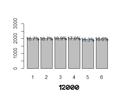 So, the empirical distribution doesn’t really start to
settle around the theoretical distribution until I input 12,000 trials. Probably
not the answer that most people would hope for. Granted, I bet a standard game
probably includes 500 – 1000 dice rolls, so really that is only one or two
dozen games.
So, the empirical distribution doesn’t really start to
settle around the theoretical distribution until I input 12,000 trials. Probably
not the answer that most people would hope for. Granted, I bet a standard game
probably includes 500 – 1000 dice rolls, so really that is only one or two
dozen games.
Okay, that’s way more than enough for one day. Will start
working on a post discussing the mathematical side of probabilities as
mentioned above. Until then, keep praying to the dice gods if that’s your
thing!
Notes on Excel functions and R code:
Excel: Random D6 generation: =RANDBETWEEN(1,6)
Counting “=#”: =COUNTIF(A1:A6,"=1")
"R" basic programCounting “=#”: =COUNTIF(A1:A6,"=1")
Rstudio (makes R have a much nicer interface):
"dice" package
Simulation Code, only need to input first two lines once. To alter number or trials, see red text. Also need to adjust the y axis increments accordingly, approximately 1/4 of number of experiments.
p.die <- rep(1/6,6)
die <- 1:6
s <- table(sample(die, size=6000, prob=p.die, replace=T))
lbls = sprintf("%0.1f%%", s/sum(s)*100)
barX <- barplot(s, ylim=c(0,1500))
text(x=barX, y=s+10, label=lbls)
No comments:
Post a Comment